housing-price-predictor

Home » Projects » Housing Price Predictor » Jupyter Code

Jupyter Notebook Model Code and Approach:

import numpy as np # linear algebra
import pandas as pd # data processing, CSV file I/O (e.g. pd.read_csv)

import os
for dirname, _, filenames in os.walk('data'):
    for filename in filenames:
        print(os.path.join(dirname, filename))

data\data_description.txt
data\sample_submission.csv
data\test.csv
data\train.csv

# Loading Training and Test Data
train_data_file = "data/train.csv"
test_data_file = "data/test.csv"

X = pd.read_csv(train_data_file, index_col='Id')
X_test = pd.read_csv(test_data_file, index_col='Id')

X.dropna(axis=0, subset=['SalePrice'], inplace=True)
y = X.SalePrice              
X.drop(['SalePrice'], axis=1, inplace=True)

X.head()

	MSSubClass	MSZoning	LotFrontage	LotArea	Street	Alley	LotShape	LandContour	Utilities	LotConfig	...	ScreenPorch	PoolArea	PoolQC	Fence	MiscFeature	MiscVal	MoSold	YrSold	SaleType	SaleCondition
Id
1	60	RL	65.0	8450	Pave	NaN	Reg	Lvl	AllPub	Inside	...	0	0	NaN	NaN	NaN	0	2	2008	WD	Normal
2	20	RL	80.0	9600	Pave	NaN	Reg	Lvl	AllPub	FR2	...	0	0	NaN	NaN	NaN	0	5	2007	WD	Normal
3	60	RL	68.0	11250	Pave	NaN	IR1	Lvl	AllPub	Inside	...	0	0	NaN	NaN	NaN	0	9	2008	WD	Normal
4	70	RL	60.0	9550	Pave	NaN	IR1	Lvl	AllPub	Corner	...	0	0	NaN	NaN	NaN	0	2	2006	WD	Abnorml
5	60	RL	84.0	14260	Pave	NaN	IR1	Lvl	AllPub	FR2	...	0	0	NaN	NaN	NaN	0	12	2008	WD	Normal

5 rows × 79 columns

# Checking columns

low_cardinality_columns = [col for col in X.columns if X[col].nunique() < 10 and X[col].dtype == "object"]
num_columns = [col for col in X.columns if X[col].dtype in ["int64", "float64"]]

required_columns = low_cardinality_columns + num_columns
high_cardinality_columns = [col for col in X.columns if col not in required_columns]

print(required_columns)
print("Dropped_columns", high_cardinality_columns)

['MSZoning', 'Street', 'Alley', 'LotShape', 'LandContour', 'Utilities', 'LotConfig', 'LandSlope', 'Condition1', 'Condition2', 'BldgType', 'HouseStyle', 'RoofStyle', 'RoofMatl', 'MasVnrType', 'ExterQual', 'ExterCond', 'Foundation', 'BsmtQual', 'BsmtCond', 'BsmtExposure', 'BsmtFinType1', 'BsmtFinType2', 'Heating', 'HeatingQC', 'CentralAir', 'Electrical', 'KitchenQual', 'Functional', 'FireplaceQu', 'GarageType', 'GarageFinish', 'GarageQual', 'GarageCond', 'PavedDrive', 'PoolQC', 'Fence', 'MiscFeature', 'SaleType', 'SaleCondition', 'MSSubClass', 'LotFrontage', 'LotArea', 'OverallQual', 'OverallCond', 'YearBuilt', 'YearRemodAdd', 'MasVnrArea', 'BsmtFinSF1', 'BsmtFinSF2', 'BsmtUnfSF', 'TotalBsmtSF', '1stFlrSF', '2ndFlrSF', 'LowQualFinSF', 'GrLivArea', 'BsmtFullBath', 'BsmtHalfBath', 'FullBath', 'HalfBath', 'BedroomAbvGr', 'KitchenAbvGr', 'TotRmsAbvGrd', 'Fireplaces', 'GarageYrBlt', 'GarageCars', 'GarageArea', 'WoodDeckSF', 'OpenPorchSF', 'EnclosedPorch', '3SsnPorch', 'ScreenPorch', 'PoolArea', 'MiscVal', 'MoSold', 'YrSold']
Dropped_columns ['Neighborhood', 'Exterior1st', 'Exterior2nd']

# Defining Pipeine

from sklearn.compose import ColumnTransformer
from sklearn.pipeline import Pipeline
from sklearn.impute import SimpleImputer
from sklearn.preprocessing import OneHotEncoder
from xgboost import XGBRegressor
from sklearn.model_selection import cross_val_score


numerical_transformer = SimpleImputer(strategy="constant")

categorical_transformer = Pipeline(steps=[
    ("imputer", SimpleImputer(strategy="constant")),
    ("one_hot_encoding", OneHotEncoder(handle_unknown='ignore'))
])

preprocessor = ColumnTransformer(
    transformers=[
        ("num", numerical_transformer, num_columns),
        ("categorical", categorical_transformer, low_cardinality_columns)
    ])

def get_scores(n_estimators, learning_rate):
    xgb_regressor_model = XGBRegressor(n_estimators=n_estimators,
                                       learning_rate=learning_rate,
                                       random_state=0,
                                       n_jobs=4)

    model_pipeline = Pipeline(steps=[
        ("preprocessor", preprocessor),
        ("model_run", xgb_regressor_model)
    ])
    
    scores = -1 * cross_val_score(model_pipeline, X, y, cv=3, scoring="neg_mean_absolute_error")
    
    return scores.mean()

# Training the model and finding the appropriate values

results = {}

for i in range(8, 13):
    for j in range(3):
        results[(100*i, 0.04 + 0.01*j)] = get_scores(100*i, 0.04 + 0.01*j)

import matplotlib.pyplot as plt
from mpl_toolkits.mplot3d import Axes3D
import math

print(results)

x_axis = list(each[0] for each in results)
y_axis = list(each[1] for each in results)
error = list(results[each] for each in results)

fig = plt.figure(figsize=(6, 6))
ax = fig.add_subplot(111, projection='3d')
ax.scatter(x_axis, y_axis, error,
           linewidths=1, alpha=.7,
           edgecolor='k',
           s = 200,
           c=error)
plt.show()

min_mae = math.inf
res = None
for each in results:
    if results[each] < min_mae:
        min_mae = results[each]
        res = each
        
print(res, min_mae)

{(800, 0.04): 16426.066360313274, (800, 0.05): 16644.35843671902, (800, 0.06): 16616.37067847101, (900, 0.04): 16420.687485278242, (900, 0.05): 16644.81792217291, (900, 0.06): 16614.745626356205, (1000, 0.04): 16421.153885892607, (1000, 0.05): 16645.025433508446, (1000, 0.06): 16615.373328139787, (1100, 0.04): 16422.57223537278, (1100, 0.05): 16647.211379823897, (1100, 0.06): 16615.751751592063, (1200, 0.04): 16424.282063426614, (1200, 0.05): 16647.23725164021, (1200, 0.06): 16616.21497778621}

png

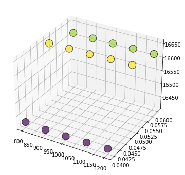
(900, 0.04) 16420.687485278242

# Thus the minimum error is n_esitimators = 900 and learning_rate = 0.04
# Setting up final model using the required params
import pickle


xgb_regressor_model = XGBRegressor(n_estimators=res[0],
                                   learning_rate=res[1],
                                   random_state=0,
                                   n_jobs=4)

model_pipeline = Pipeline(steps=[
    ("preprocessor", preprocessor),
    ("model_run", xgb_regressor_model)
])

# Fitting the input and predicting the results
model_pipeline.fit(X, y)

# Saving the model to load it quickly in case we want to reuse it.
pickle.dump(model_pipeline, open("housing_price_model.pkl", "wb"))

# In case you want to predict without training the model again
# model_pipeline = pickle.load(open("housing_price_model.pkl", "rb"))

# Model Prediction
preds = model_pipeline.predict(X_test)

#Saving Output

output = pd.DataFrame({"Id": X_test.index, "SalePrice": preds})
output.to_csv("submission.csv", index=False)

output.head()

	Id	SalePrice
0	1461	126472.671875
1	1462	155542.046875
2	1463	187986.968750
3	1464	190310.859375
4	1465	188251.093750

# Kaggle_Score: 14997.99107
# https://www.kaggle.com/competitions/home-data-for-ml-course/leaderboard#

housing-price-predictor

Contents:

Contents:

Jupyter Notebook Model Code and Approach: